Christopher J. Kimmer, Ph.D.
IU Southeast Informatics
iSci
the informatics of scientific computing
Next: Approximating the Quasiperiodic Surface Up: Introduction Previous: Differential Geometry of Triangulated
Error in Minimizing Discrete Surfaces
Little has been published or is rigorously known about the approximation of a minimal surface by a triangulated surface. Fundamental questions such as ``Does a discrete surface with h ≡ 0 guarantee a surface with H ≡ 0 ?'' or ``Does a discrete surface with h ≠ 0 preclude a nearby continuous surface from having H ≡ 0 ?'' are not answered. The most convincing numerical evidence for the existence of a minimal surface based on triangulated approximations is to demonstrate that a discrete surface is sufficiently minimal over a series of successively-refined triangulations with decreasing edge length, but it is not clear how best to define ``sufficiently minimal'' and not proven that even this demonstration guarantees a surface's existence.
More usefully, Underwood[ 53 ] has studied the problem of how well a triangulated surface can approximate a minimal surface. In regards to the first question asked above, Underwood finds that one may place conditions on a triangulated surface (which may be verified in principle using the Evolver) that guarantee that there is a minimal surface nearby. Unfortunately, rigorous error measurements require several orders of magnitude more faces per triangulated surface than can be currently fit into a calculation. (A computer with 512 MB of memory can only efficiently process about 100,000 facets, and this is also prohibitively slow since minimizations with so many degress of freedom are glacial.)
Fortunately, Underwood finds that it is rather simple to illustrate that the
second question's answer may be ``No,
h
≠
0
does not rule out
H
= 0
''. For a given triangulation of a minimal surface, even
one with vertices exactly on the surface,
h
will in
general not be zero
whenever the triangulation is not equiangular around the
vertex. The discrete mean curvature at a vertex
v
is still
essentially the average of
the principal curvatures over the faces of the triangulation sharing
v
, and the effect of the non-equiangular triangulation is to weight
one principal curvature more than the other leading to nonzero mean
curvature that is directly proportional to the geometric mean of the principal
curvatures of the nearby minimal surface (i.e. the square root of the
absolute value Gaussian curvature). Furthermore,
this error is the same for another triangulation about
v
having smaller edge lengths but the same vertex angles about
v
.
Consequently, the relevant issue to explore is how small must
h
or
![]() h
i
2
h
i
2
![]() be before one has confidence that the mean
curvature estimate will be within the bounds of this inevitable error. In
other words, the only possible numerical test is to measure how small
h
is compared to the principal curvatures.
be before one has confidence that the mean
curvature estimate will be within the bounds of this inevitable error. In
other words, the only possible numerical test is to measure how small
h
is compared to the principal curvatures.
In order to measure
h
relative to the principal curvatures, the
principal curvatures must be obtained from the triangulated surface.
For the case of a continuous surface,
the scale of the principal curvatures can be found from the absolute
value of the
Gaussian curvature,
|
K
| = |
k
1
k
2
|
, so that when
H
is small, a principal
curvature's absolute value is roughly
![]() .
For a triangulated surface, the Gaussian
curvature is well-defined and
simply computed from the angle deficit about a vertex
i
; if a
triangulation about the vertex has inner angles
{
θj
}
,
the integral of Gaussian curvature over the area associated with
vertex
i
,
.
For a triangulated surface, the Gaussian
curvature is well-defined and
simply computed from the angle deficit about a vertex
i
; if a
triangulation about the vertex has inner angles
{
θj
}
,
the integral of Gaussian curvature over the area associated with
vertex
i
,
![]() is
is
|
|
( 50 ) |
The evolution of the triangulation can yield an estimate for
|
|
( 51 ) |
Finally, taking the ratio of these quantities provides a quantitative measure of how almost-minimal a surface is at each vertex i
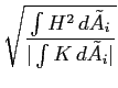 =
=
 .
.
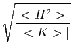
This measure puts h on the scale of the principal curvatures and would, of course, be zero for a true minimal surface. The only proviso is that points where K ≡ 0 should be avoided. Such points are known as flat points, and although there are infinitely many of them in the quasiperiodic minimal surface (every 3- and 5-fold saddle point has one), they are isolated from one another (see Reference [ 23 ], p. 76). The average of the Γi error measure over the vertices of a triangulation, < ≅ > , will be used to characterize the minimality of the relaxed surface patches associated with the quasiperiodic minimal surface since it is not proven that a nearby minimal surface exists.
Further conditions that ensure a triangulation is ``going in the right direction'' towards a minimal surface can be stated. Since the integral of mean curvature along an edge is the product of the edge length and the dihedral angle between the two faces sharing the edge, the dihedral angle and edge length should tend toward zero as a triangulation is refined. For some triangulations evolved by minimizing the integral of discrete mean curvature squared, it is difficult to keep the edge lengths uniformly decreasing over successive refinements. For this reason the longest edge length over successive refinements of a triangulation is a very good indicator of the quality of a triangulation.
In the case of periodic minimal surfaces where the existence of a surface has been rigorously proven, a triangulation with the correct topology can be evolved in order to gain reasonable error estimates for a surface's curvature and total area. These estimates can then be applied to other surfaces where minimality may not be known beforehand. It is worthwhile to note that many periodic minimal surfaces may be evolved in other numerically more stable ways with correspondingly better numerical cuvature properties. For instance, balance periodic minimal surfaces are often evolved by constraining a surface patch to separate regions of equal volume. This constraint stabilizes the surface patch and allows one to minimize the area functional rather than the integral of squared mean curvature[ 54 ].
To gain a sense of what ``zero mean curvature'' means for a triangulated
minimal surface, the curvature properties of three discrete periodic
minimal surfaces are summarized
in Tables
4.1
,
4.2
, and
4.3
.
Each of these tables lists the area, maximum dihedral angle, and longest
edge length at the minimum of
E
h
over successive refinements of
the starting triangulation for each surface
along with the number of vertices, edges,
and faces of the triangulations.
Of the most relevance to the study of the quasiperiodic
minimal surfaces is the properties of the Neovius surface which can
be formed by cutting the
Ψ
(
x
) = 0
isosurface with a specific,
rationally-oriented 3-plane[
25
].
Data for
the evolution of Neovius' surface are shown in Table
4.1
while
Table
4.2
contains the data for the Schwarz P surface. Data
for the Schwarz D surface are in Table
4.3
.
| Refinement | A |
|
V | E | F | θmax | l max | < ≅ > | |
| 1 | .3536 | 8.18e-16 | 5 | 8 | 4 | 2.98e-8 | .866 | 7.8e-6 | |
| 2 | .3000 | 3.47e-16 | 13 | 28 | 16 | .660 | .444 | 1.3e-8 | |
| 3 | .2940 | 1.05e-7 | 41 | 104 | 64 | .427 | .318 | 1.6e-5 | |
| 4 | .2929 | 8.23e-9 | 145 | 400 | 256 | .245 | .204 | 4.5e-5 | |
| 5 | .2926 | 5.42e-11 | 545 | 1568 | 1024 | .142 | .137 | 4.0e-6 | |
| 6 | .2926 | 2.07e-7 | 2113 | 6208 | 4096 | .075 | .100 | 1.1e-6 |
| Refinement | A |
|
V | E | F | θmax | l max | < ≅ > |
| 1 | .1969 | 4.50e-15 | 12 | 28 | 16 | .295 | .343 | 1.4e-7 |
| 2 | .1958 | 5.31e-13 | 41 | 104 | 64 | .188 | .235 | 2.9e-6 |
| 3 | .1955 | 1.01e-12 | 145 | 400 | 256 | .107 | .118 | 1.4e-7 |
| 4 | .1954 | 1.12e-8 | 545 | 1568 | 1024 | .052 | .074 | 5.9e-6 |
| 5 | .1954 | 5.04e-8 | 2113 | 6208 | 4096 | .029 | .047 | 3.6e-5 |
| Refinement | A |
|
V | E | F | θmax | l max | < ≅ > |
| 1 | .3214 | 3.80e-15 | 15 | 30 | 16 | .283 | .332 | 6.5e-8 |
| 2 | .3202 | 3.92e-14 | 45 | 108 | 64 | .146 | .209 | 4.4e-10 |
| 3 | .3199 | 5.45e-13 | 153 | 408 | 256 | .075 | .131 | 2.9e-8 |
| 4 | .3198 | 1.63e-12 | 561 | 1584 | 1024 | .037 | .082 | 7.3e-5 |
| 5 | .3198 | 5.67e-11 | 2145 | 6240 | 4096 | .019 | .041 | 5.5e-7 |
The net result that may be gleaned from these tables is that the integral of squared mean curvature generally increases monotonically over successive refinements; a finer triangulation does not lead to lower values of the approximate Willmore energy. The areas of the surfaces are much better behaved; not very many faces are needed in an evolved triangulation to ensure that the area has converged to three decimal places, say. The surface patches for these periodic minimal surfaces consistently demonstrate the smallest < ≅ > values and hence the best numerical curvature properties of the surfaces studied here. Other topologically more complicated surfaces that have lots of handles, say, demonstrate areas that are also converged, but are not as well-converged as these examples. Also, the descent to ``zero mean curvature'' is rather rapid for the periodic minimal surfaces. The mean curvature typically decreases by several orders of magnitude once an an energy valley or basin of attraction for a nearby minimum has been reached; it is possible that the energy landscape of the evolutions by discrete mean curvature are riddled with barriers or plateaus in some cases.
Next: Approximating the Quasiperiodic Surface Up: Introduction Previous: Differential Geometry of Triangulated