Christopher J. Kimmer, Ph.D.

IU Southeast Informatics

The Critical Surface

The critical surface (see Section 2.2.4) itself provides the most stringent available tests on the viability of this method for constructing a minimal surface. Regardless of the topology of the critical surface itself, the properties of a minimal surface in physical space place severe restrictions on the critical surface's projection into perp space. The observation that bubbles are surfaces of nonzero constant mean curvature, and therefore not minimal, implies that physical space can contain no bubbles. Bubbles are formed when Sheng's inner critical ``sphere'' is crossed, so this sphere must fuse with the rest of the critical surface to form a structure with vanishing thickness as t → 0 .

When the critical surface's projection into perp space has no thickness, all the local topology changes associated with crossing that piece of critical surface happen simultaneously and no bubbles will be in physical space. In this limit of zero thickness, the critical surface can be viewed as a kind of acceptance domain for the minimal surface in physical space. Topology jumps that modify the minimal surface in physical space without destroying its minimality occur whenever the cut plane crosses the critical surface, in the same way that phason jumps occur in a quasiperiodic tiling when the cut crosses an ADs boundary.

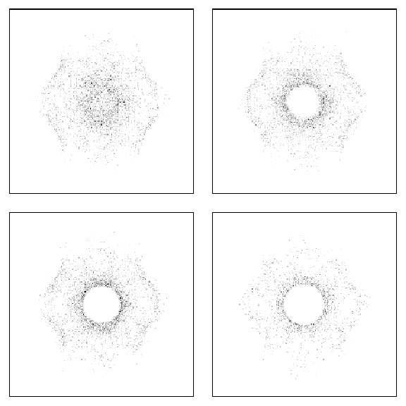
A silhouette of the critical surface in perp space can be obtained from the real space data by a three-step process. First, constrast is introduced to highlight grid points with small Ψ ( x ) since only these grid points nearest the Ψ ( x ) = 0 isosurface are potentially relevant to the critical surface. The contrast is introduced into the data by defining a function f _i for each grid point x _i with Ψ ( x _i ) ≡ ψ_i

where γ is an adjustable parameter. The second step of the procedure to image the critical surface relies on the observation that grid points with small values of ψ_i (where the contrast f _i is greatest) that are nearest to the critical surface will tend to cluster on planes roughly corresponding to x _⊥ = constant . Finally, a mirror plane in perp space, say the x - y plane orthogonal to the two-fold axis along the z direction, is selected and discretized into an N x N grid of points, and the { ψ_i } are projected into perp space. Points lying in the mirror plane are assigned to their nearest perp space grid point, and all points corresponding to a given perp space grid point have their values of { f _i } summed. The FCC grid points nearest the critical surface will be projected onto planes in perp space, or in the case of the mirror plane in perp space, lines of high contrast against a weaker background.

This procedure is carried out, and the evolution of the critical surface contained in a 6D BCC Voronoi cell about the origin as t is lowered for n = 32 is shown in Figure  2.7 . As the amplitude of the dominant star of three-fold wavevectors increases, the 5D surface loses its isotropy with respect to para and perp space, and kinks begin to form in the surface in perp space. The envelope of these kinks is the central hole in the plots in Figure  2.7 , and this hole increases in size initially. As t is further decreased and the surface's topology has stabilized, the hole is no longer growing. By far the most interesting development is that the critical surface is developing facets at t = .075 and much more clearly at t = .05 (See Figure  2.5 ). The smaller values of n studied by Sheng, and indeed results through n = 30 , show the boundary of the excluded region in the mirror plane to be nearly circular, and the n = 32 results provide the first departure from this picture.

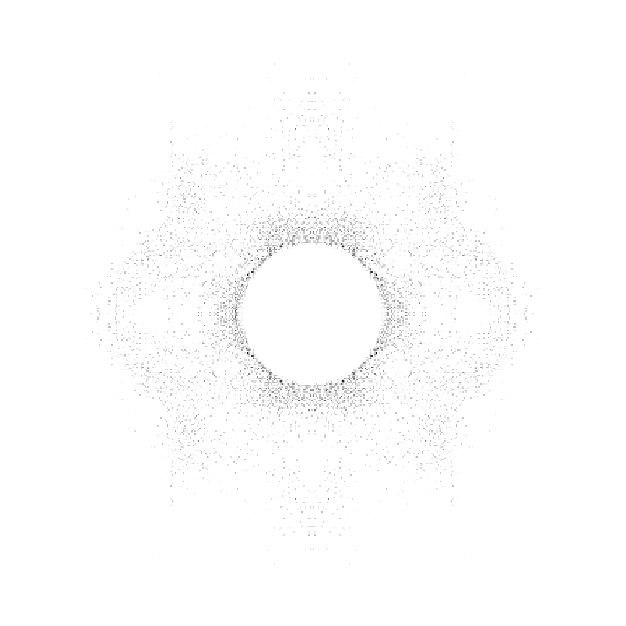
It is difficult to say more about what kind of polyhedron to associate with this faceted critical surface, but the orientation of the facets seen in the mirror plane views are not consistent with a triacontahedron since vertices or edges on two-fold axes are clearly seen. A vertex of the critical surface does lie on the bisector of 5-fold lattice vectors { ½ ½ ½ ½ ½ } , and this agrees with the scale of the critical surface indicated in Reference [ 25 ]. It is also worth noting that this procedure to visualize the critical surface does not have very good resolution, so it is not clear whether the inner or outer envelope of the critical surface is viewed in this procedure. Most likely, it is some combination of the two. Sheng's conjecture that the outward appearance of the critical surface projected into perp space is a triacontahedron cannot be verified or refuted. Numerical studies at larger values of n are necessary to provide a more detailed view of the critical surface than the n = 32 data provide.

Chris Kimmer 2011-06-01

Valid XHTML | CSS