Christopher J. Kimmer, Ph.D.
IU Southeast Informatics
iSci
the informatics of scientific computing
Numerical Results
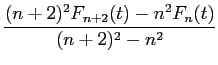
The results for the free-energy evolution as the anisotropy parameter t is decreased are shown in Figure 2.4 where the energy has been rescaled following Equation 2.13 . It is expected that, for a given value of t , the leading term in the difference between the free energy in the continuum limit F ∞ ( t ) and the free energy F n ( t ) computed at a particular value of n is proportional to n-2 . Linear fits of the computed energies at a given value of t for two consecutive values n and n + 2 allow extrapolation to the expected free energy F ∞ n ( t ) in the limit n → ∞ :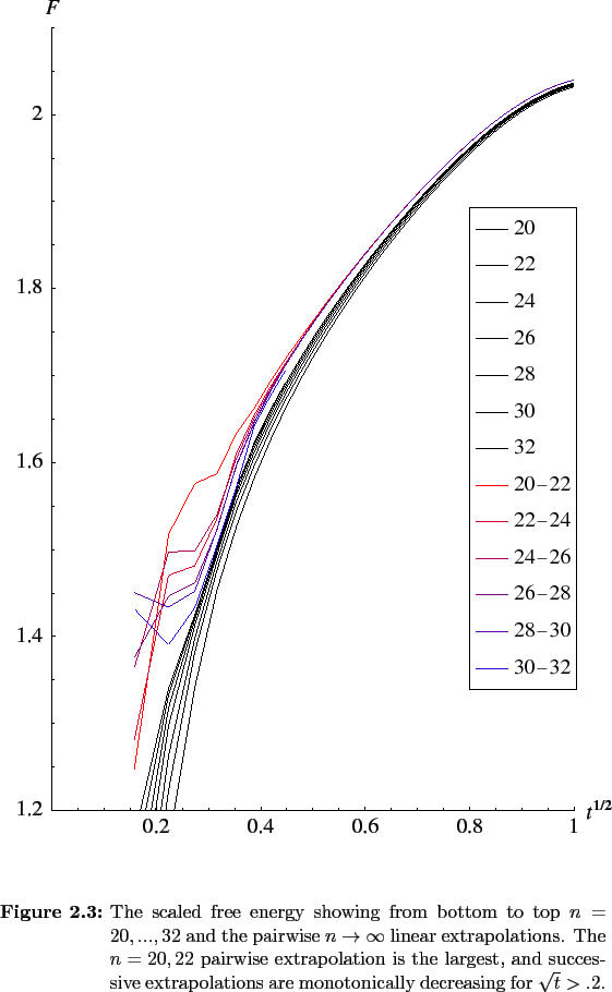
F
∞
n
(
t
) =
 .
.
|
( 21 ) |
These pairwise extrapolations are also shown in Figure 2.4 . Finally, the series of estimations F 20 ∞ ( t ), F 22 ∞ ( t ),... F 30 ∞ ( t ) are least squares fit to provide the best estimate of the value of F ∞ ( t ) , and these values as function of t are in turn fit to the form of Equation 2.13 to yield fitting coefficients of A || = 1.2 and V || = 1.0 . The value of A || exactly agrees with Sheng's while she found V || to be 1.3 . The pairwise linear extrapolation of the n = 30 and 32 pairs of data sets reveals that the convergence of the energies for each n value is well behaved for t ≥ 0.075 . For t < 0.075 the free energies cannot be considered to be converged, although the topology and form of the interface as determined by the amplitudes of the low-order Fourier modes are stable down to t values at least an order of magnitude smaller.
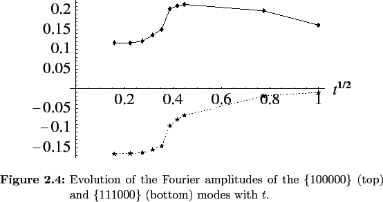
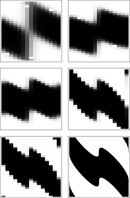
The higher resolution energies have revealed no surprising behavior as demonstrated by the Fourier transforms of the results, shown in Figure 2.5 . The agreement with Sheng's results is good, but as n increases the amplitude of the three-fold star of wavevectors increases relative to that of the five-fold star. This does not affect the topology of the 5D surface, for as the interface's evolution in Figure 2.6 (see next section) illustrates, there is still excellent agreement between the real space data and Equation 2.14 .
|
Chris Kimmer 2011-06-01