Christopher J. Kimmer, Ph.D.

IU Southeast Informatics

iSci

the informatics of scientific computing

Methodology

Higher resolution numerical studies allow smaller values of t to be probed, and the desired limit of infinite stretch in perp space may be more closely approached. Higher resolution studies can also reveal if the topology defined by Equation 2.14 remains stable at smaller t values, and most importantly, the critical surface may be studied in more detail.

To study the functional's behavior, the method referred to by Sheng as the ``real space method'' is used. The free energy functional is discretized on a 6D FCC lattice containing n ⁶ /2 lattice points per cubic unit cell. (A 6D simple cubic lattice would be much simpler to implement, but its nearest-neighbor vectors have equal projections onto the para and perp spaces. In constrast, the nearest-neighbor vectors of the 6D FCC lattice have different length projections in the two subspaces, and the projection of the gradient terms into para and perp space can be implemented.

The discretization of Equation 2.8 involves replacing the bulk energy terms with a sum over lattice points, and the gradient terms are replaced with finite difference expressions. As noted in Reference [ 25 ], the FCC lattice contains two stars of 30 two-fold nearest neighbor vectors, { v ¹ _i } ≡ {110000} and { v ² _i } ≡ {1 $\bar{{1}}$ 0000} . Inflating the vectors { v ¹ _i } yields the set { v ² _i } ; the interchange of the two sets of vectors corresponds to the interchange of para and perp space. The { v ¹ _i } have parallel and perp space magnitudes of

$\displaystyle {\frac{{\vert v^1_\parallel\vert^2}}{{\vert v^1_\perp\vert^2}}}$ = $\displaystyle {\frac{{\frac{6}{5}-\frac{2}{5}\tau}}{{\frac{4}{5}+\frac{2}{5}\tau}}}$ = τ^-2

( 16 )

while the corresponding ratio is reciprocal for the { v ² _i } . The discretization over an FCC grid with n ⁶ /2,( n even) points per simple cubic unit cell means that a given grid point will have nearest neighbor separations given by n^-1 { v ^j _i } .

Only symmetry-inequivalent (under the 240 element orbit of Y _h coupled with the BCC translation generating the sign change in Ψ( x ) ) grid points { x _i } are kept, and the free energy for grid resolution n is the sum over grid points written as

F = $\displaystyle {\frac{{2}}{{n^6}}}$ $\displaystyle \sum_{i}^{}$ a _i ( f ⁿⁿ _i + (1 - ψ_i² ) ² )

( 17 )

with a _i denoting the length of the orbit of x _i under the action of the 240-element icosahedral group Y _h with a BCC translation, and ψ_i ≡ Ψ ( x _i ) . The gradient terms depend only on the values at a grid point and its nearest neighbors to first order and are given by

f ⁿⁿ _i = $\displaystyle {\frac{{n^2}}{{20}}}$ ( τ κ_∥ - $\displaystyle {\frac{{1}}{{\tau}}}$ κ_⊥ ) $\displaystyle \sum_{j}^{}$ [ Ψ ( x _i + v ¹ _j ) - ψ_i ] ² +

$\displaystyle {\frac{{n^2}}{{20}}}$ ( τ κ_⊥ - $\displaystyle {\frac{{1}}{{\tau}}}$ κ_∥ ) $\displaystyle \sum_{j}^{}$ [ Ψ ( x _i + v ² _j ) - ψ_i ] ² ,

( 18 )

where κ_∥ and κ_⊥ are parameterized by κ_∥ = k ₀ t and κ_⊥ = k ₀ t ² with k ₀ = .02 . The computer memory used to store the nearest neighbor data structure for the computation of the gradient term is the limiting factor in determining how large a grid may be simulated in a timely manner. An SGI Onyx with 4GB of RAM can fit the data structure for n = 30 into memory, and larger grids are only possible through the use of disk space.

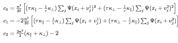
With this discretized form of the free energy, one may simulate the system as a set of interacting points and minimize the free energy by sequentially minimizing the energy density locally at each symmetry-inequivalent point and iterating until the energy has suitably converged to a minimum. The free energy density at a given point is a quartic function of the value of the order parameter at the point and its sixty nearest neighbors and can be written as

1 + c ₀ + c ₁ ψ_i + c ₂ ψ_i² + ψ_i⁴

( 19 )

with the coefficients c _i given by

$\displaystyle \singlespacing$ $\displaystyle \begin{array}{l} c_0 = \frac{n^2}{20} \left[ (\tau \kappa_\paral... ... c_2 = \frac{3 n^2}{2} (\kappa_\parallel + \kappa_\perp ) - 2 \end{array}$ $\displaystyle \normalspacing$

( 20 )

so that c ₂ is independent of the grid point. Newton's method is used to quickly minimize Equation 2.18 at each grid point.

Grid resolutions of n = 26, 28, 30, and 32 are used, which results in up to 2,269,824 symmetry inequivalent grid points; the maximum number of points used by Sheng was approximately 400,000. The resulting discretely-sampled order parameter can be Fourier transformed to compute the low-order Fourier terms that characterize the topology of the structure. All other necessary visualization can be carried out with the real space data itself in order to preserve the maximal amount of information.

Chris Kimmer 2011-06-01

cjkimmer -at- ius.edu

Valid XHTML | CSS