Christopher J. Kimmer, Ph.D.

IU Southeast Informatics

iSci

the informatics of scientific computing

Algebraic Structure of the Inflation Matrices

The possible entries for columns of inflation matrices have already been listed in Table 3.2 , and Appendix A contains an example of the derivation of an inflation matrix specific to a choice of inflation rules. Beyond specific choices of inflation rules, the structure of the matrices themselves is extremely interesting and sheds some light on the properties of these tilings.

A general inflation matrix for any of these tilings constructed by any choice of inflation rules can be written down based on knowledge of the relative tile frequencies. For instance, if one knows that half of the T ₁ tetrahedra inflate one way and half another, the entry for T ₁ tetrahedra in an inflation matrix is the average of the entries for these two possible ways listed in Table 3.2 . More abstractly, a generalized inflation matrix can be written as an average over the entries in Table 3.2 weighted by the relative frequencies of each particular inflation of a tile. These frequencies are not in general known without knowledge of the inflation matrix itself, but some interesting properties of the tiling turn out not to depend on the relative tile frequencies.

Headway can be gained by considering the form of the weighted average. Combinatorially, there are only three ways to inflate a T ₁ tetrahedron and two ways to inflate all the other tiles. The number of relative frequencies that must be specified to construct an inflation matrix is only the number of combinatorially inequivalent ways to inflate a tile, so it is less than the number of ways considered in the above paragraph. A general inflation matrix can be written as

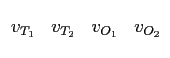
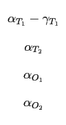
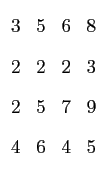
$\displaystyle \singlespacing$ $\displaystyle \cal {M}$ ≡ $\displaystyle \left(\vphantom{ \begin{array}{rrrr} v_{T_1} & v_{T_2} & v_{O_1} & v_{O_2} \end{array} }\right.$ $\displaystyle \begin{array}{rrrr} v_{T_1} & v_{T_2} & v_{O_1} & v_{O_2} \end{array}$ $\displaystyle \left.\vphantom{ \begin{array}{rrrr} v_{T_1} & v_{T_2} & v_{O_1} & v_{O_2} \end{array} }\right)$ $\displaystyle \normalspacing$

( 37 )

with the entries for each tile v _i written as the weighted average over the entries of Table 3.2 :

$\displaystyle \singlespacing$ v _{T
₁} = α_T₁ $\displaystyle \left(\vphantom{ \begin{array}{c} 3 2 2 4 \end{array} }\right.$ $\displaystyle \begin{array}{c} 3 2 2 4 \end{array}$ $\displaystyle \left.\vphantom{ \begin{array}{c} 3 2 2 4 \end{array} }\right)$ + β_T₁ $\displaystyle \left(\vphantom{ \begin{array}{c} 4 1 5 2 \end{array} }\right.$ $\displaystyle \begin{array}{c} 4 1 5 2 \end{array}$ $\displaystyle \left.\vphantom{ \begin{array}{c} 4 1 5 2 \end{array} }\right)$ + γ_T₁ $\displaystyle \left(\vphantom{ \begin{array}{c} 5 0 8 0 \end{array} }\right.$ $\displaystyle \begin{array}{c} 5 0 8 0 \end{array}$ $\displaystyle \left.\vphantom{ \begin{array}{c} 5 0 8 0 \end{array} }\right)$ ≡ α_T₁ A _{T
₁} + β_T₁ B _{T
₁} + γ_T₁ C _{T
₁} $\displaystyle \normalspacing$

( 38 )

subject to the constraint that α_T₁ + β_T₁ + γ_T₁ = 1 to normalize the relative frequencies for this tile. Similar entries can be written for the other tiles, each of which inflate in only two combinatorially distinct ways. Using the same notation as in the T ₁ case introduces the relative frequencies α_i , β_i , i ∈ { T ₂ , O ₁ , O ₂ } and the column vectors A _i , B _i , i ∈ { T ₂ , O ₁ , O ₂ } . To be specific, fix the { A _i , B _i } by order they are listed in Table 3.2 . The normalization condition implies that β_i = 1 - α_i , implying 5 degrees of freedom in the specification of $\cal {M}$ .

As shown in Section 3.4, all the rearrangements between two combinatorially distinct τ² inflations of a tile correspond to adding or subtracting $\cal {F}$ ≡ (1, - 1, 3, - 2) from the inflation matrix column entries in Table 3.2 . Specifically, there are the relations

A _{T ₁} + $\displaystyle \cal {F}$	=	B _{T ₁}
C _{T ₁} - $\displaystyle \cal {F}$	=	B _{T ₁}
A _{T ₂} + $\displaystyle \cal {F}$	=	B _{T ₂}
A _{O ₁} + $\displaystyle \cal {F}$	=	B _{O ₁}
A _{O ₂} + $\displaystyle \cal {F}$	=	B _{O ₂} .

( 39 )

This single flip $\cal {F}$ along with the normalization of the relative frequencies allows the general inflation matrix of Equation 3.11 to be written independently of the { β_i } as

$\displaystyle \singlespacing$ $\displaystyle \cal {M}$ = ( B _{T
₁} , B _{T
₂} , B _{O
₁} , B _{O
₂} ) + (1, -1, 3, -2) ^. $\displaystyle \left(\vphantom{ \begin{array}{c} \alpha_{T_1} - \gamma_{T_1} ... ... \alpha_{T_2} \alpha_{O_1} \alpha_{O_2} \end{array} }\right.$ $\displaystyle \begin{array}{c} \alpha_{T_1} - \gamma_{T_1} \alpha_{T_2} \alpha_{O_1} \alpha_{O_2} \end{array}$ $\displaystyle \left.\vphantom{ \begin{array}{c} \alpha_{T_1} - \gamma_{T_1} ... ... \alpha_{T_2} \alpha_{O_1} \alpha_{O_2} \end{array} }\right)$ , $\displaystyle \normalspacing$

( 40 )

and the matrix with columns given by the { B _i } is written as

$\displaystyle \singlespacing$ $\displaystyle \cal {M}$ ₀ ≡ $\displaystyle \left(\vphantom{ \begin{array}{cccc} 3 & 5 & 6 & 8 2 & 2 & 2 & 3 2 & 5 & 7 & 9 4 & 6 & 4 & 5 \end{array} }\right.$ $\displaystyle \begin{array}{cccc} 3 & 5 & 6 & 8 2 & 2 & 2 & 3 2 & 5 & 7 & 9 4 & 6 & 4 & 5 \end{array}$ $\displaystyle \left.\vphantom{ \begin{array}{cccc} 3 & 5 & 6 & 8 2 & 2 & 2 & 3 2 & 5 & 7 & 9 4 & 6 & 4 & 5 \end{array} }\right)$ . $\displaystyle \normalspacing$

( 41 )

Equation 3.14 shows that any general inflation matrix has some constant core associated with it plus a variable part that depends on the relative frequencies of the combinatorially inequivalent ways of re-tiling an inflated tile.

The matrix $\cal {M}$ ₀ has a zero eigenvalue with eigenvector $\cal {F}$ , so the decomposition of the general inflation matrix in Equation 3.14 isolates the $\cal {F}$ -direction in the 4-dimensional tile space from $\cal {M}$ ₀ . Consequently, $\cal {F}$ must be an eigenvector of the general inflation matrix $\cal {M}$ , with an eigenvalue dependent on the values of the { α_i , γ_T₁ } given by ( α_T₁ - γ_T₁ - β_T₂ +3 β_O₁ -2 β_O₂ ) . A left eigenvector corresponding to the eigenvalue τ⁶ of $\cal {M}$ ₀ and $\cal {M}$ is the vector $\cal {V}$ whose entries are proportional to the volume of each tile. Since left and right eigenvectors of different eigenvalues are orthogonal, $\cal {V}$ ^. $\cal {F}$ = 0 ; in other words, the two tile flips $\cal {F}$ represents conserve volume. Additionally, all the tile flips discussed in Section 3.4 change at most one vertex along the same edge, so the vertex fraction in the volume the tile flips are confined to does not change. Consequently, the $\cal {F}$ vector is also orthogonal to the vector $\cal {W}$ representing the number of vertex fraction in each tile ( $\cal {W}$ = ( ${\frac{{2}}{{15}}}$ , ${\frac{{1}}{{5}}}$ , ${\frac{{3}}{{20}}}$ , ${\frac{{23}}{{120}}}$ ) ).

Manipulating inflation matrices is only arcana until the vertex density of a tiling constructed with inflation rules is computed. The density can be written in terms of the vectors $\cal {V}$ and $\cal {W}$ discussed above along with the right eigenvector χ/2 of $\cal {M}$ with eigenvalue τ⁶ which gives the relative frequencies of tiles

ρ = $\displaystyle {\frac{{{\cal W}\cdot \chi}}{{{\cal V}\cdot \chi}}}$ .

( 42 )

Since $\cal {W}$ is orthogonal to $\cal {F}$ , it may be written as the sum of the three left eigenvalues of $\cal {M}$ orthogonal to $\cal {F}$ , in particular $\cal {W}$ = w ₀ $\cal {V}$ + w ₁ x {other eigenvectors} , which states that one of the left eigenvectors is still $\cal {V}$ and the others are included in the sum. The vector χ/2 is orthogonal to all of the left eigenvectors except $\cal {V}$ with which it shares an eigenvalue, so $\cal {W}$ ^. χ/2 = w ₀ $\cal {V}$ ^. χ/2 . This implies that ρ is constant:

ρ = w ₀ = $\displaystyle {\frac{{3}}{{20}}}$ + $\displaystyle {\frac{{1}}{{10}}}$ τ .

( 43 )

It is not particularly staggering that a family of tilings have invariant vertex density; it has been remarked that several two-dimensional families of tilings have this property. What is interesting is that the eigenvector χ/2 is not constant; it depends on the relative weights of the { α_i , γ_T₁ } . Consequently, the tile frequencies change while still giving rise to the same vertex density.

It is clear that any one pruning operation $\cal {P}$ leaves the density invariant since in the tiling picture the pruning operation forces tile rearrangements that are stable with respect to both the volume and vertex fraction per tile vectors. However, it is less clear that the density has to be stable with respect to successive inflations where making a particular choice of inflation rule at one step affects the form of the tiling at successive inflation steps. It has not been shown that the 4 tile rearrangements described above can be used to modify a given tiling into any arbitrary tiling constructed by these inflation rules.

Chris Kimmer 2011-06-01

cjkimmer -at- ius.edu

Valid XHTML | CSS